In this worksheet, we will examine the behavior of
different general exponential functions by comparing their graphs.
HOW TO USE THIS WORKSHEET:
As you read, graph the curves on your own graphing calculator or software.
Try changing:
the function (especially the base),
the x_min,
and the x_max.
Ask:
How did the range (the maximum and minimum y-values) change?
How did the shape of the curve change?
What does that tell me about the function?
This is the best way to get a correct gut feeling for general exponential functions!
HOW TO READ THIS WORKSHEET:
This was written using Sage (a free computer algebra software system).
To plot the function y=f(x) on the domain (x_min, x_max), we will write
plot(f(x),x_min,x_max)
To plot the graphs of f(x) and g(x) on the same axes, we will write
plot(f(x),x_min,x_max,linestyle='dashed')+plot(g(x),x_min,x_max,linestyle='solid')
We can tell the two functions apart because the graph of y=f(x) will be a dashed curve,
and the graph of y=g(x) will be a solid curve.
|
|
PART I.
To begin, let's look at exponential functions y=a^x
where the base a>1.
Notice that as the base of the exponential increases,
the function grows faster (as we move from smaller x-axis values to larger x-axis values).
|
|
plot(2^x,0,10,linestyle='solid')+plot(e^x,0,10,linestyle='dashed')+plot(3^x,0,10,linestyle='dotted')
|
|
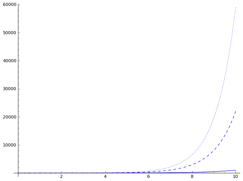
It is clear by looking at the graph that e^x and 3^x both increase quickly toward infinity.
It is less clear from the above graph what the function 2^x does.
In fact, 2^x also increases quickly toward infinity.
To see this, lets graph the slowest growing of the three (y=2^x) on a slightly longer interval of the x-axis:
|
|
plot(2^x,0,15,linestyle='solid')
|
|
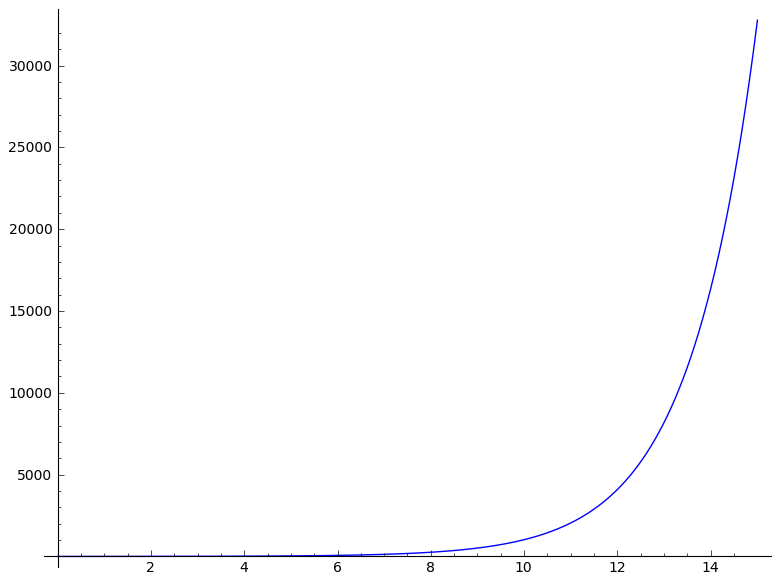
Notice that the curve y=2^x does grow toward infinity very quickly,
it just takes longer for the curve to really take off.
|
|
PART II.
Now, let's look at what happens to the graph of y=a^x
in three cases:
a>1,
a=1, and
0<a<1
|
|
plot(1.001^x,-250,1000,linestyle='dashed')+plot(1^x,-250,1000,linestyle='solid')+plot(.999^x,-250,1000,linestyle='dotted')
|
|
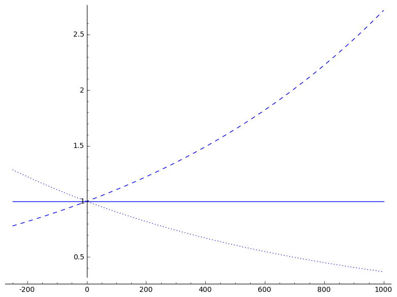
Note that as x goes to infinity:
a^x goes to infinity when a>1,
a^x is constant when a=1, and
a^x goes to 0 when 0<a<1
|
|
PART III.
Finally, let's look at exponential functions y=a^x
where the base 0<a<1.
Notice that when the base of the exponential is bigger,
the function drops off to 0 faster (as we move from small x-values to large x-values).
|
|
plot(.1^x,-.5,10,linestyle='dotted')+plot(.5^x,-.5,10,linestyle='dashed')+plot(.9^x,-.5,10,linestyle='solid')
|
|
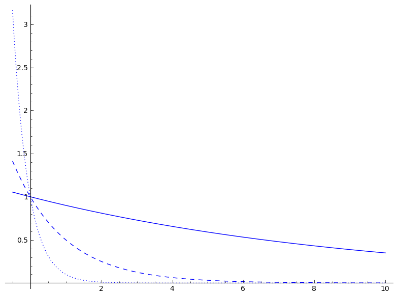
In the above graph, it is easy to see that .1^x and .5^x both approach 0, first quickly and then evening off.
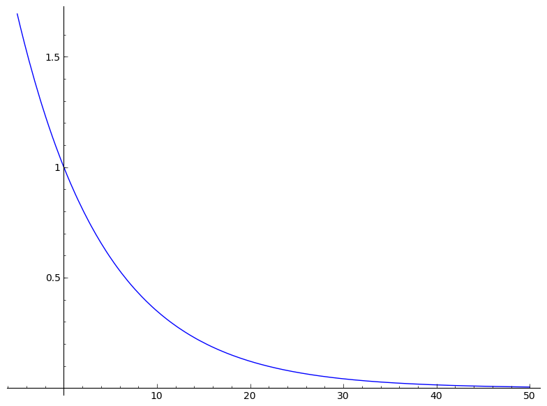
By graphing y=.9^x on a larger interval, we can see that .9^x also approaches 0, first quickly and then evening off.
|
|
plot(.9^x,-5,50,linestyle='solid')
|
|
|
|